|
A Roger’s Rabbit Hole White Paper
|
Why memory capacity, bandwidth and allocation determine practical local LLM performance
By Roggie D | November 2026
A CyberTron hardware case study. Nov. 16, 2026.
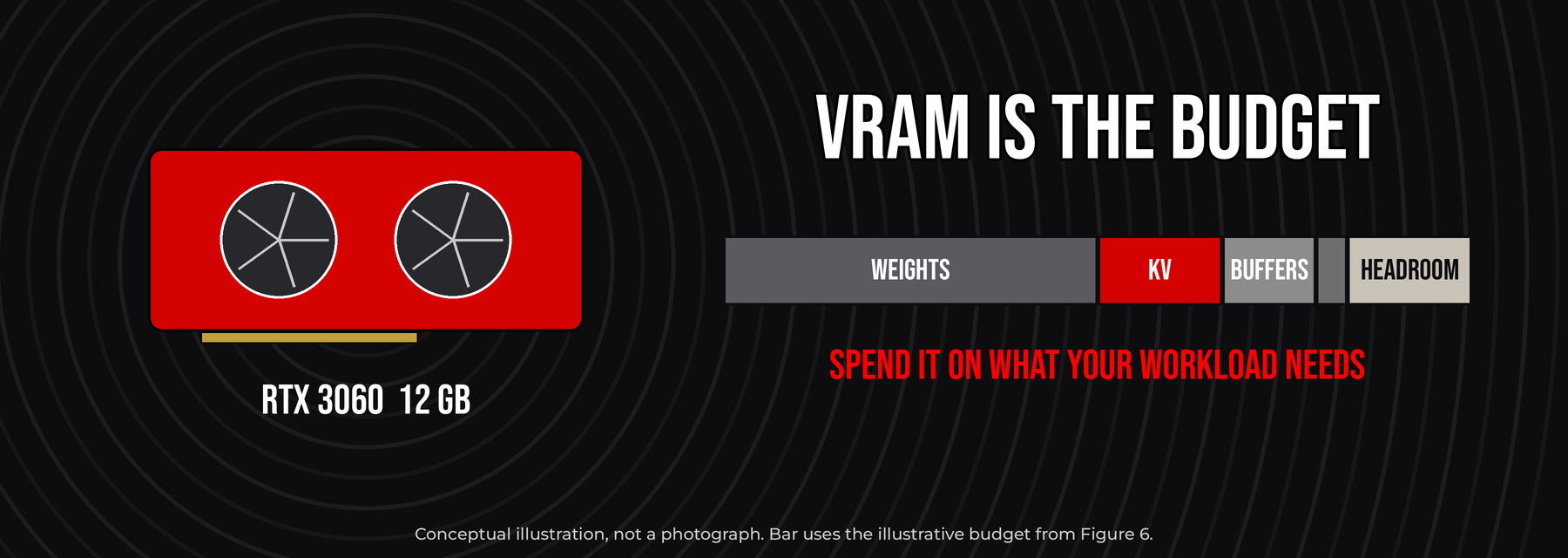
A conceptual sketch, not a photo: 12 GB of VRAM is a budget, and every model, context and request spends some of it.
| |
WHO THIS IS FOR
Written for local AI enthusiasts, homelab operators, systems engineers, IT administrators, AI developers and small organizations trying to figure out what a graphics card will really do for local language models.
|
| |
HOW I LABEL THE NUMBERS
CyberTron numbers in this paper are historical results from my project records. Calculated figures and illustrative scenarios are labeled as such. I didn’t run any new live benchmarks for this paper.
|
Graphics cards get sold on compute throughput and gaming performance. If you run local language models, the number that often decides what you can do is how much GPU memory you have. A model doesn’t just have to exist on disk. Its weights, attention cache, working buffers and other runtime allocations all have to fit somewhere in the memory hierarchy. When they don’t fit in the card’s video RAM (VRAM), the inference engine has to shrink allocations, move things around, push work onto the CPU or refuse the job. Each of those changes latency and throughput in ways a CUDA core count can’t explain.
This paper lays out a practical way to budget VRAM. It explains the difference between memory capacity and memory bandwidth, works through weight and KV cache sizing, and looks at context length, concurrent requests, quantization and multi-GPU tradeoffs. My example is CyberTron, a resource-constrained box built on an AMD FX-8300, 32 GB of DDR3 and an NVIDIA RTX 3060 12 GB. Its partial-offload history shows why keeping more of a model on the GPU can speed things up, and it also exposes the limits of an aging CPU and host memory.
VRAM is a scarce operating budget. Capacity decides which model configurations can live on the card. Bandwidth and compute decide how fast they run once they’re there. Neither spec tells the story on its own.
1. The big misunderstanding about AI GPUs
|
1.1 Gaming performance isn’t LLM inference performance
Games lean on graphics throughput, frame rendering and latency-sensitive graphics pipelines. Autoregressive transformers do repeated matrix math over learned model parameters and cache attention state from token to token. Both use parallel computing, but they hit different bottlenecks. A GPU that’s excellent for graphics may not have the memory a given language model needs. That can produce a surprising reversal: on that particular workload, a less powerful GPU with more VRAM can beat a faster GPU that’s forced to lean on host memory.
Table 1. Compute versus VRAM for one 11 GB working set (hypothetical example).
| Characteristic |
Hypothetical GPU A |
Hypothetical GPU B |
| Compute capacity |
High |
Moderate |
| VRAM |
8 GB |
16 GB |
| Model working set |
11 GB |
11 GB |
| Full resident placement |
No |
Potentially yes |
| Likely decision |
Change the model or offload |
Benchmark full GPU residency |
1.2 Capacity versus bandwidth
Capacity is how much working data the GPU can hold. Bandwidth is how fast data moves between VRAM and the processing units. Lots of memory doesn’t guarantee speed, and high bandwidth can’t hold a model that’s bigger than the card. Real inference speed also depends on the architecture, arithmetic precision, runtime kernels, batching and the balance between prompt prefill and token decoding.
1.3 Why VRAM is the real currency
Every active model spends part of the GPU memory budget. Longer context spends more cache. More concurrent requests spend more. Multimodal encoders and temporary buffers spend more. You can trade compute, quality or latency for lower VRAM use, but none of those tricks makes the budget go away. So a practical design starts by accounting for what gets consumed, not by comparing a download’s file size to the number on the GPU box.
2. GPU memory architecture and the cost of moving data
|
On the RTX 3060 12 GB, the GDDR6 memory delivers about 360 GB/s of nominal bandwidth [2]. The link between the motherboard and the card is far narrower. Theoretical one-way PCIe x16 bandwidth is about 8 GB/s for PCIe 2.0, 15.75 GB/s for PCIe 3.0 and 31.5 GB/s for PCIe 4.0 [10]. Those peak rates aren’t interchangeable measurements of what software actually achieves: GPU memory traffic and host-to-device transfers do different jobs.
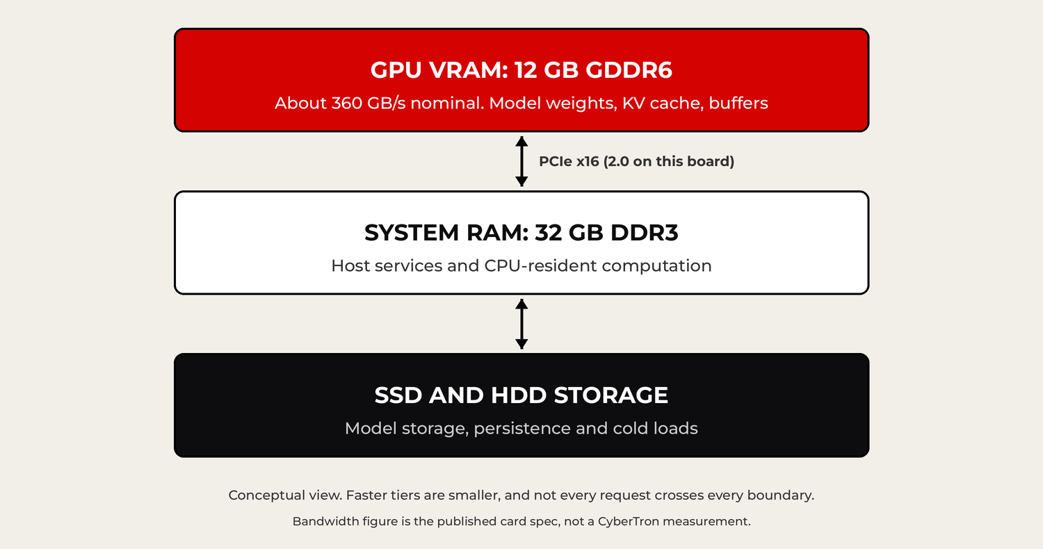
Figure 1. VRAM, system RAM and storage serve distinct roles. Not every request crosses every boundary.
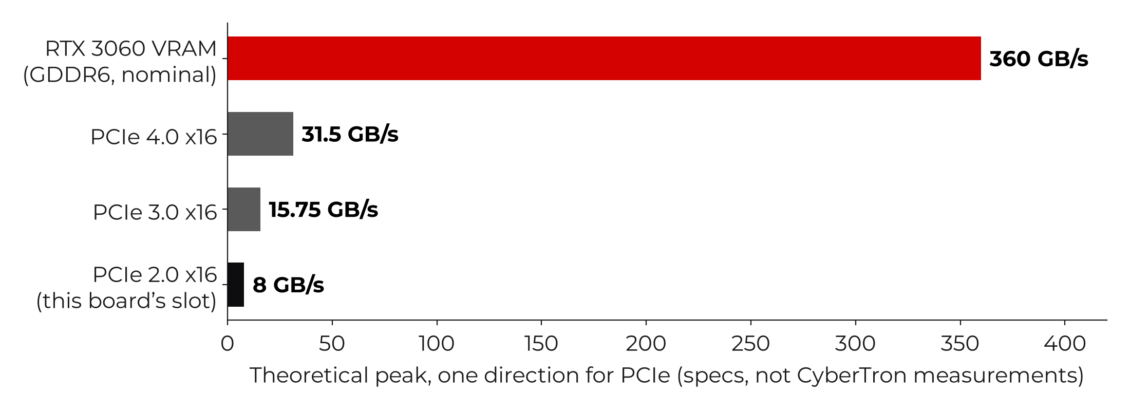
Figure 2. Nominal and theoretical bandwidth compared. GPU VRAM and PCIe are different interfaces, and these values are not end-to-end benchmarks.
CyberTron still runs on a PCIe 2.0-era AM3+ platform, even though the RTX 3060 supports newer PCIe signaling. A GPU-resident model can still do useful inference, because decoding token after token doesn’t mean reloading all the model weights over PCIe. Host-offloaded layers, frequent tensor transfers and memory oversubscription are what make the old platform’s limits show.
3. What actually takes up GPU VRAM
|
For planning, I use this:
|
M_GPU ≈ M_weights + M_KV + M_workspace + M_other
|
Those terms cover model weights, attention key and value state, temporary buffers and other resident allocations. Runtime accounting can differ: reservations, cached allocations, physical commitments and per-process reports don’t always agree.
3.1 Model weights and precision
For a dense model with P parameters stored at b effective bits per parameter, a simplified baseline estimate is:
|
M_weights ≈ P × b ÷ 8 bytes
|
For an 8B dense model, that works out to 32 GB at 32 bits, 16 GB at 16 bits, 8 GB at 8 bits and 4 GB at 4 bits (calculated). Format metadata, per-block scales, mixed precision and architecture details change real GGUF file sizes and actual runtime allocations.
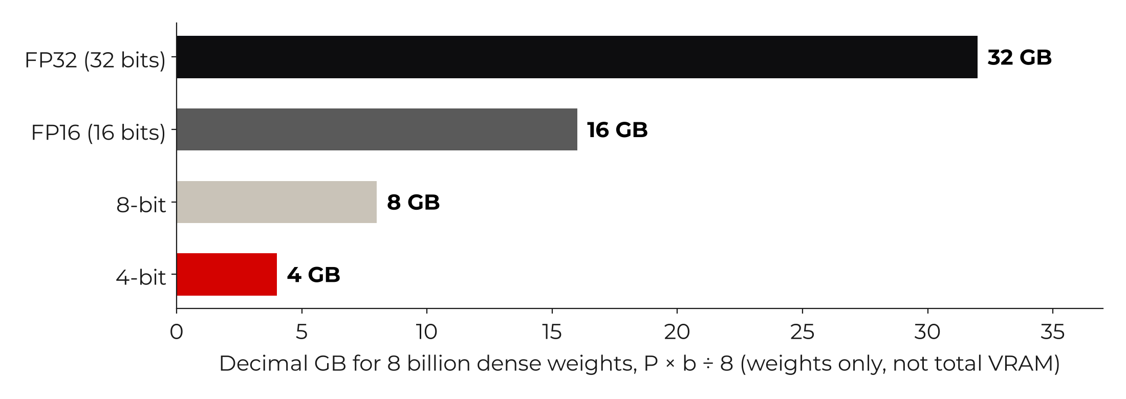
Figure 3. Idealized storage for 8 billion dense-model weights (calculated). Not a total VRAM estimate.
3.2 Quantization: trading precision for memory
GGUF formats such as Q4_K_M, Q5_K_M and Q8_0 store weights at reduced precision using implementation-specific block structures. Quantization can let a model fit on a consumer GPU, but it may change numerical accuracy and task results, and it can change kernel performance too [7]. The right unit of evaluation is the exact artifact: the quantization, model revision, context configuration and inference engine. A label like “4-bit” on its own isn’t enough.
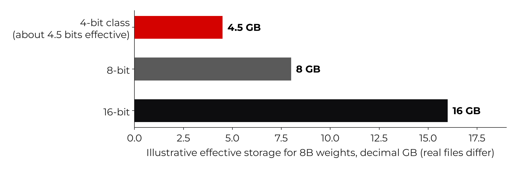
Figure 4. Illustrative effective weight storage for 8B parameters. Actual artifacts differ.
3.3 KV cache and long context
Autoregressive attention caches keys and values so the model doesn’t keep recomputing every earlier attention projection. For a conventional transformer with L layers, T cached tokens, H_KV KV heads, head dimension D and B bytes per cached value, the approximate full-attention storage is:
|
M_KV = 2 × L × T × H_KV × D × B
|
The factor of two covers the key and value tensors. Grouped-query attention, sliding-window attention, compressed or latent attention, cache quantization and allocator behavior can all change the result.
Take an illustrative architecture with 32 layers, eight KV heads, 128-dimension heads and an FP16 cache. That’s 128 KiB per cached token, so 4K of context needs about 0.5 GiB of KV memory, 8K needs 1 GiB, 16K needs 2 GiB, 32K needs 4 GiB and 64K needs 8 GiB (calculated). These aren’t universal requirements for any named model.
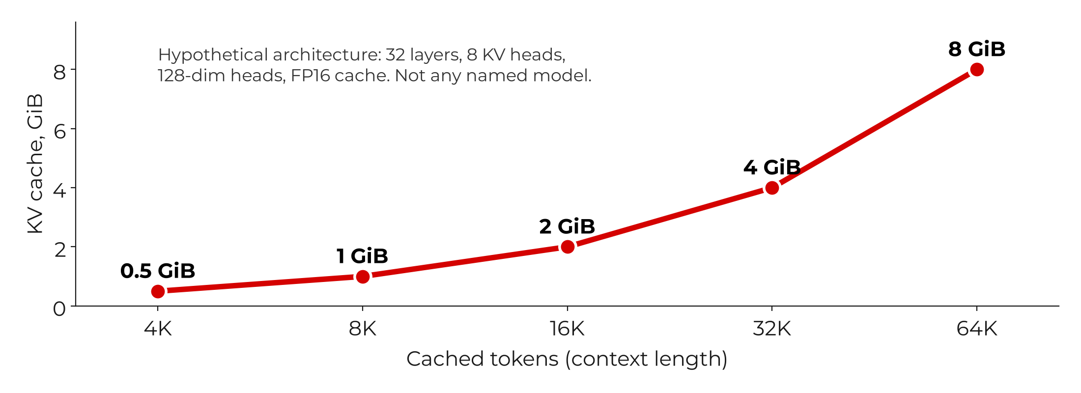
Figure 5. Hypothetical FP16 KV cache growth with context length for one specified architecture (calculated).
3.4 Concurrency and shared cache pressure
Concurrent requests usually need their own KV state even when they share model weights. At a high level, KV use scales roughly with the sum of active sequence lengths, but prefix sharing, paging, slot scheduling, reuse and preemption can change the allocations. Serving engines such as vLLM document preemption under KV cache pressure: it preserves request progress but can force recomputation and longer latency [5]. Single-user measurements alone can’t tell you what a team will need.
4. Building a defensible VRAM budget
|
Say a 12 GB GPU runs a model configured with 6.0 GB of resident weights, 2.0 GB of cache, 1.5 GB of workspaces and 0.5 GB of other allocations. That’s an estimated 10 GB allocated, with 2 GB of nominal headroom. This budget is deliberately illustrative. It is not a measured CyberTron allocation, and allocation behavior and context reserve policies differ by runtime.
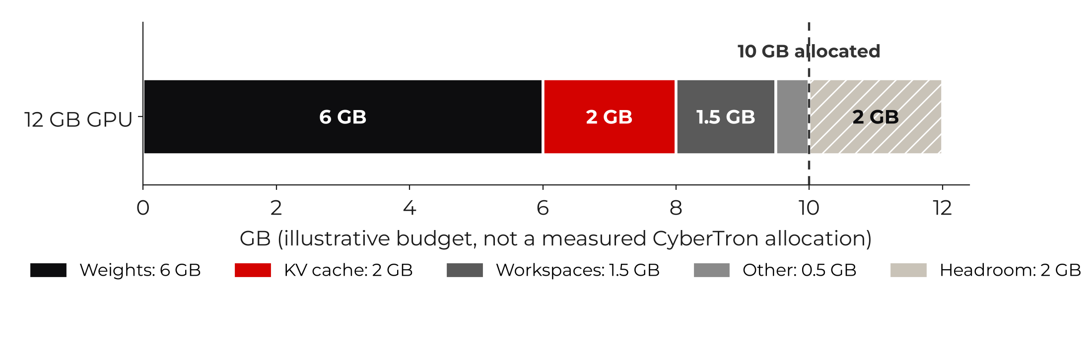
Figure 6. Illustrative partition of a 12 GB GPU: 10 GB allocated plus 2 GB of headroom.
4.1 Worked example: planning model memory
Take an 8B dense model at an assumed effective 4.5 bits per weight: 8 × 4.5 ÷ 8 = 4.5 decimal GB of idealized weights. Add a hypothetical 16K KV cache of 2 GiB (about 2.15 GB) and a 1.5 GB runtime allowance. The estimate comes to about 8.15 GB (calculated). The cache architecture and the allowance are examples, not attributes of a specific 8B model, so check the estimate against an actual model load.
A useful admission rule: the estimated total working set plus a deliberate free margin has to be less than the usable device capacity. Don’t treat an 11.9 GB estimate as a dependable 12 GB deployment. Driver reservations and transient allocations can make it fail right at the limit.
5. Bandwidth: why more memory isn’t always faster
|
A simplified bandwidth roofline for low-batch decoding is:
|
R_memory ≤ B_effective ÷ W_token
|
R_memory is the token rate memory bandwidth allows, B_effective is the achieved bandwidth and W_token is the effective bytes read per token. Suppose a hypothetical decode process moves an effective 6 GB of data from GPU memory for every token, at an ideal 360 GB/s. The arithmetic caps it at 60 tokens per second (360 ÷ 6, calculated). Real performance differs with achieved bandwidth, repeated attention reads, dequantization, execution kernels, batching and compute overhead. This illustrates the mechanism. It isn’t a CyberTron benchmark.
5.1 Prefill versus decode
Prefill can process many prompt tokens together and is often more compute-sensitive. Decode usually generates tokens one after another in single-user sessions and is often more bandwidth-sensitive. Batching can improve overall utilization but raise an individual request’s latency. Benchmarks need to report both stages to explain what a user actually experiences.
Table 2. What to measure, and why users notice.
| Measurement |
What it represents |
Why users notice |
| Prefill throughput |
Prompt tokens processed per second |
Delay before a long input is ready |
| Time to first token (TTFT) |
End-to-end time until the first token |
How responsive it feels at the start |
| Decode throughput |
Generated tokens per second |
How fast the answer streams |
| End-to-end latency |
Complete time for a request |
Overall usability of the service |
6. The CyberTron hardware case study
|
CyberTron is my budget local AI box. Here’s its documented configuration [8]:
Table 3. CyberTron’s documented configuration (historical project records).
| Subsystem |
Documented CyberTron configuration |
| CPU |
AMD FX-8300 (legacy AM3+ platform) |
| Motherboard |
ASUS M5A78L-M family |
| RAM |
32 GB DDR3 |
| GPU |
NVIDIA RTX 3060, 12 GB GDDR6 |
| GPU predecessor |
NVIDIA GTX 1060, 6 GB |
| Storage |
512 GB OS SSD, an added 1 TB SSD and a legacy HDD |
| Inference stack |
Ollama, llama.cpp, Open WebUI |
| Operating system |
A current Ubuntu Server LTS release |
The original GTX 1060 had 6 GB of VRAM. Moving to the RTX 3060 doubled the room for resident models to 12 GB and added newer CUDA and Tensor Core capability [1]. That combination mattered because model placement, not just the CPU’s age, set much of what the box could practically run. The full upgrade story, costs included, is in my last white paper, Building AI on Aging Hardware.
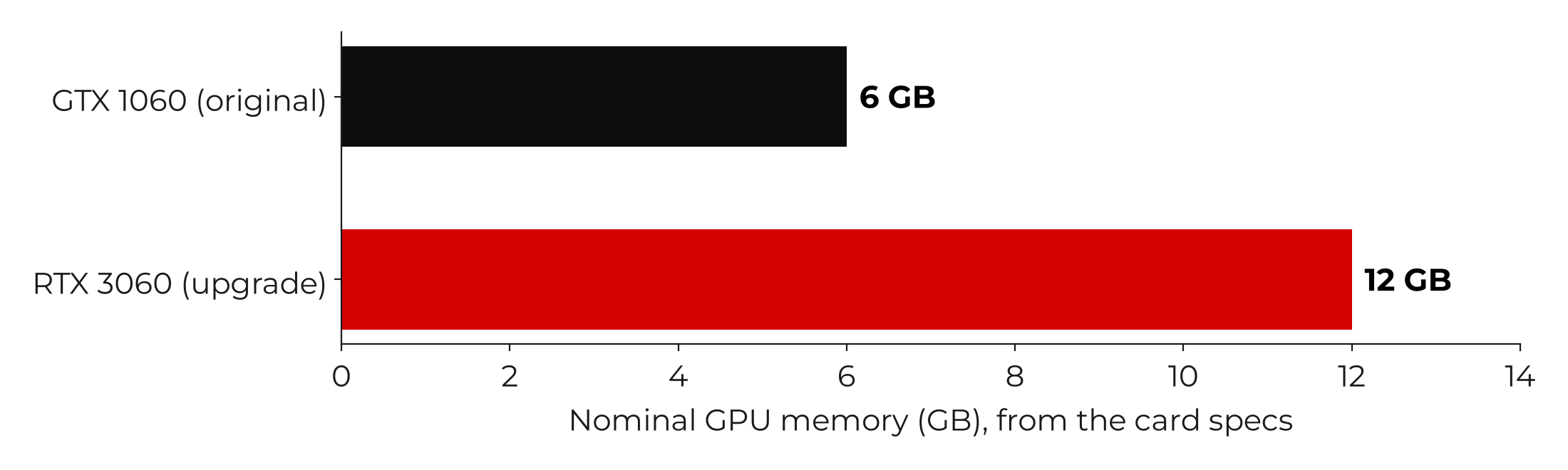
Figure 7. Documented CyberTron upgrade: VRAM capacity doubled from 6 GB to 12 GB.
6.1 Evidence: smaller models that stayed on the GPU
My historical CyberTron runs recorded full GPU placement for Qwen3 8B [12] at tested 4K, 8K and 16K contexts. Qwen3 14B [13] was observed at about 9.6 GB of VRAM with full GPU placement in selected 4K, 8K and 12K tests. Those observations came from particular model and runtime configurations. They don’t guarantee that every similarly named artifact or context setting will fit.
| |
FROM MY BENCH
WHY QWEN3 14B FIT AND THE 35B DIDN’T
On paper, Qwen3 14B at about 9.6 GB left roughly 2.4 GB of a 12 GB card for everything else. That’s 12 minus 9.6, my arithmetic, not measured headroom. The 35B model’s file alone was about 21.7 billion bytes, bigger than the whole card before a single byte of cache or buffers. One lived on the GPU. The other had to share the work with an FX-era CPU and DDR3.
|
6.2 Evidence: the bigger partial-offload experiment
One recorded test used a 35B-total, 3B-active mixture-of-experts model, a community build based on Qwen3.6-35B-A3B [9], run at 4-bit (Q4_K_M). To be clear, it is not an official Qwen release. I pulled it from Hugging Face in October 2026, and it lives in my model rack. The file is around 21.7 billion bytes. Because that’s bigger than 12 GB of VRAM before any runtime overhead, the model ran split across the CPU and GPU. Recorded generation throughput was 4.35 tokens per second with 8 layers offloaded to the GPU, 6.15 at 12 and 7.09 at 16. Those settings weren’t a rigorously normalized benchmark series. They show the direction of the benefit I saw as more layers moved onto the GPU.
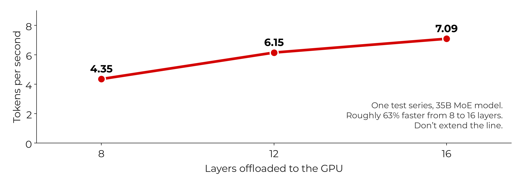
Figure 8. Historical CyberTron GPU layer offload observations for the 35B community build. Not a general performance forecast.
Going from 8 to 16 GPU-offloaded layers lined up with about 63% more recorded generation speed in this specific series (7.09 ÷ 4.35, calculated). The FX CPU and DDR3 stayed in the critical path, which is why partial offload could still be far slower than a smaller model that fit entirely on the GPU. How much data moves, which layers go where, the runtime settings and where the KV cache lives all matter.
These are the same offload numbers I reported in Building AI on Aging Hardware. The different 35B figures in my first white paper came from separate runs, not from this series.
6.3 Mixture-of-experts: active compute isn’t stored memory
Mixture-of-experts (MoE) models route each token through selected expert networks. The parameters actually used for a token can be far fewer than the model’s total parameter count. That can cut per-token arithmetic, but the inactive experts still take up storage and have to be reachable when they’re selected. A 35B-total MoE model with roughly 3B active parameters doesn’t use GPU memory like an ordinary 3B dense model. Size MoE deployments from the total artifact size and runtime placement, then measure actual memory traffic and speed.
7. CPU offload, system RAM and PCI Express
|
Hybrid CPU and GPU execution widens the range of model sizes you can run, but it moves layers or tensors into host memory and onto the CPU. For many transformer workloads, CPU-side work on the FX-8300 can’t match the RTX 3060’s acceleration. A useful way to think about it:
|
time per token ≈ GPU work + CPU work + device transfers + synchronization and other costs
|
Real runtimes can overlap parts of that work. On old systems, getting layers off the CPU may be worth more than chasing theoretical GPU compute.
7.1 Why storage isn’t substitute VRAM
An SSD speeds up cold loads and model switching. It doesn’t come close to the working speed of the GDDR6 memory on the GPU itself. Memory mapping and paging can head off immediate out-of-memory errors, but the cost in performance and system stability depends heavily on access patterns. A big SSD model library is useful for a model rack. Just don’t confuse it with room for models that are resident at the same time.
8. Multi-GPU: more cards don’t automatically pool memory
|
Two 12 GB GPUs don’t automatically look like one uniform 24 GB allocation to every inference engine. The software has to explicitly split model layers or tensors across devices. With layer or pipeline partitioning, each card holds its assigned weights and usually the matching cache. Tensor parallelism may pass partial results back and forth often and can add a lot of interconnect overhead. Consumer cards on PCIe without high-speed peer links may lose efficiency at small batch sizes.
Table 4. Multi-GPU and hybrid options compared.
| Configuration |
Potential benefit |
Principal tradeoff |
| One 24 GB GPU |
Single-device residency and simpler scheduling |
Purchase cost and available architectures |
| Two 12 GB GPUs |
Can split larger models if the runtime supports it |
Inter-GPU communication and uneven distribution |
| 12 GB GPU plus host RAM |
Lower cost if the hardware is already owned |
CPU, RAM and PCIe penalties in the critical path |
| Two independent GPU services |
Serve separate models or requests |
No shared capacity for one model |
The llama.cpp project documents several multi-GPU split modes, including automatic placement across GPUs, custom split proportions and an experimental tensor-parallel mode [4]. Exact flags depend on the revision. A multi-GPU recommendation should start from a verified topology and runtime, not from adding up the VRAM numbers on the stickers.
9. The model rack and GPU residency policy
|
A storage-backed model rack can keep lots of specialized GGUF artifacts on hand while loading only the models the current tasks need. I made the case for model racks in Bigger Isn’t Always Smarter. A sensible routing strategy picks a small, fast general assistant for interactive work, a coder model for programming, an embedding model for retrieval and a larger specialized model only when it’s needed. On a 12 GB card, the scheduler has to control residency, model unloading, context allocations and concurrent requests to avoid oversubscription.
For throughput, keep a small number of frequently used models resident if their combined working sets truly fit. For flexibility, keep alternatives on SSD and accept the model-switch delay. Operationally, those are different service-level objectives, and neither one wins everywhere.
10. A practical way to choose a GPU
|
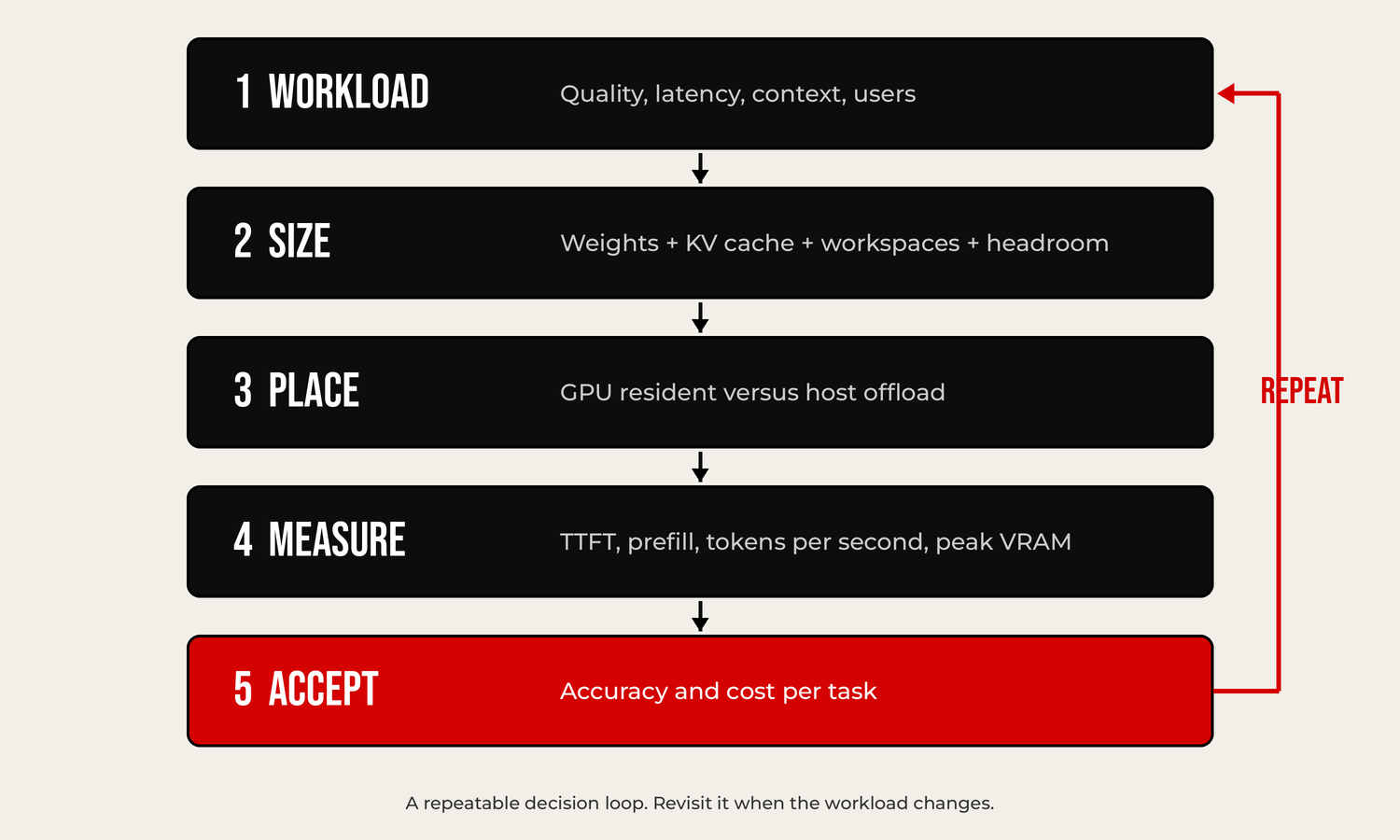
Figure 9. A repeatable decision loop for choosing and running local AI GPU hardware.
- Define the real workload: quality targets, longest realistic prompt, throughput, concurrency and privacy boundary.
- Pick candidate model artifacts and quantizations. Don’t size from parameter count alone.
- Estimate weights, context-dependent KV memory, working buffers and deliberate headroom.
- Verify support for the GPU architecture, the runtime you need, drivers and the model format.
- Test prefill speed, time to first token, decode tokens per second and answer quality under representative conditions.
- Measure sustained peak VRAM, RAM, GPU and CPU activity, temperatures and how requests fail.
- Compare total system cost, energy, maintenance and useful lifetime, not just sticker price.
10.1 Capacity tiers as planning categories
Table 5. VRAM tiers as rough planning categories, not compatibility certifications.
| VRAM tier |
Likely use cases |
Important limitation |
| 6 to 8 GB |
Small quantized models, embeddings, narrow assistants |
Shorter contexts and tighter headroom |
| 12 GB |
Many quantized 7B to 14B class configurations |
Model architecture and context affect fit |
| 16 GB |
More medium-model and cache headroom |
Large models may still offload |
| 24 GB |
Broader midsize model options, longer contexts |
Concurrency and 30B-plus sizes still need budgeting |
| 32 to 48 GB |
Larger resident models and multiuser capacity |
Compute and bandwidth still dictate throughput |
| Above 48 GB |
Higher-capacity professional and server workloads |
Power, platform and expense rise |
These tiers are deliberately approximate. A large model with unusually efficient attention can use less KV memory than a smaller model with a different architecture, and multimodal and long-context inference can flip rankings that look straightforward.
11. Diagnostics and copy-ready examples
|
Everything below is a read-only example unless noted. Run it on your own local Linux inference host. Standard user privileges are enough for the common inspection commands when the utilities are installed.
11.1 Inspect GPU capacity and utilization
nvidia-smi
nvidia-smi --query-gpu=name,memory.total,memory.used,\
utilization.gpu,temperature.gpu,power.draw --format=csv
These identify the installed NVIDIA GPUs and give a snapshot of utilization. On their own, they don’t prove which model layers are resident or how much memory a single request needs.
11.2 Inspect CPU, memory and GPU processes
lscpu
free -h
lsblk -o NAME,SIZE,TYPE,FSTYPE,MOUNTPOINTS
ollama ps
In supported Ollama versions, ollama ps shows whether a loaded model sits fully on the GPU, fully in system memory or split between the two [6] [11]. Compare that with GPU process memory, host memory and runtime logs.
11.3 A representative llama.cpp server command
# Illustrative only: verify flags with your installed llama-server --help
# MODEL_FILE stands for your own GGUF model file
llama-server -m MODEL_FILE -c 8192 -ngl 999 --host 127.0.0.1
The -ngl argument requests GPU layer offload and can be limited by automatic placement or memory fit [3]. Binding to 127.0.0.1 keeps the sample server off your network interfaces. Don’t copy this into a production service without checking version-specific syntax, authentication and your application’s requirements.
11.4 Benchmark record template
Table 6. What to record for every benchmark.
| Field |
Record |
| Model, revision, hash |
Exact artifact and checksum |
| Quantization, runtime commit |
Document both |
| GPU, driver, CUDA |
Exact hardware and software |
| Context, prompt and output tokens |
A reproducible task |
| GPU layers, KV cache type |
Placement and precision |
| TTFT, prefill, decode |
Separate latency and rates |
| Peak VRAM, RAM, power |
Sustained measurements |
| Result quality, failures |
A task acceptance criterion |
12. Security, stability and cost
|
High VRAM utilization isn’t the same as efficient operation. When memory headroom disappears, longer prompts or simultaneous requests can trigger allocation failures or scheduler preemption. Monitoring should cover request failures, memory fragmentation, model-switch time, GPU temperatures and power. Local inference also needs authenticated access, restricted management endpoints, supply-chain verification of model artifacts and a clear line between what a model suggests and any privileged automation.
A GPU purchase decision should cover the whole deployment: the graphics card, a compatible power supply and case, the remaining useful life of the host, electricity, storage, maintenance and acceptable failure recovery. An older 12 GB GPU can be an excellent value if it meets the service-level objective. A 24 GB card can pay for itself when it removes persistent CPU-offload delays or enables substantially more concurrent work. Neither choice is justified by VRAM per dollar alone.
13. Common mistakes and better approaches
|
Table 7. Common mistakes and the better engineering approach.
| Common mistake |
Better engineering approach |
| “The model file fits, so inference will fit.” |
Include KV cache, workspaces, the driver and other processes. |
| “24 GB is twice as fast as 12 GB.” |
Compare bandwidth, compute and actual placement. |
| “Two 12 GB cards always act like 24 GB.” |
Confirm supported model partitioning and its overhead. |
| “Longer context is free intelligence.” |
Measure cache size, prefill latency and real answer quality. |
| “Low-bit quantization has no accuracy cost.” |
Benchmark the exact task and the quantized artifact. |
| “A faster SSD fixes low tokens per second.” |
Profile resident versus host-executed layers. |
| “A bigger MoE active count defines memory size.” |
Budget total stored weights and actual residency. |
- VRAM capacity determines the resident working set you can actually run, not the model file size alone.
- Memory bandwidth is a major constraint for many low-batch decode workloads. Compute still matters, especially in prefill and larger batches.
- The KV cache grows with architecture, context and active sequences, so serving concurrent users takes capacity planning.
- Quantization can make a model feasible, but it has to be tested for accuracy and real runtime behavior.
- Partial CPU and GPU placement expands the model catalog but can impose severe latency penalties on legacy hardware.
- Multiple GPUs need explicit software partitioning. Capacity doesn’t pool automatically.
- CyberTron’s historical results are consistent with the advantage of GPU residency. They are not a universal ranking of models or GPUs.
The meaningful question for anybody running a local LLM isn’t just “How fast is my GPU?” It’s “Which working set can stay on my GPU, at the context and concurrency my application really needs, and how fast can it be processed, sustained?” Capacity, bandwidth, arithmetic capability, runtime implementation and service objectives form one inseparable system.
CyberTron shows why that matters. Moving from a 6 GB GTX 1060 to a 12 GB RTX 3060 changed the range of models that could stay on the GPU, without replacing the aging CPU. When larger model artifacts outgrew the VRAM, partial offload let me experiment, but it put the FX CPU and DDR3 right back in the critical path. The project shows both how much carefully chosen GPU memory is worth and where more VRAM, or a newer host, starts to make sense.
VRAM is the real currency of many local AI deployments because it buys residency, context, concurrency and flexibility. It isn’t the whole economy. Good engineering spends that currency on verified workloads, measures the returns and avoids paying for capacity or compute the applications can’t use.
Appendix A. Technical formulas
|
Weight storage, in decimal bytes:
Conventional KV cache, in bytes:
|
2 × L × T × H_KV × D_head × bytes per value
|
Planning memory:
|
weights + KV cache + workspaces + other allocations + safety headroom
|
Idealized bandwidth roofline, in tokens per second:
|
achieved memory bandwidth ÷ effective bytes moved per token
|
Approximate annual energy cost:
|
wall watts ÷ 1,000 × operating hours × electricity rate
|
Appendix B. Publication and reproducibility notes
|
Every diagram and chart in this paper was newly drawn from the values explained in the text. None of them is a screenshot of the CyberTron system, and none is a photograph. The interactive calculators from my working notes appear here as static, reproducible worked examples. Values described as hypothetical or illustrative are design examples, not verified device measurements. Hardware specs such as VRAM, memory bandwidth and PCIe rates come from manufacturers and published references, not from my bench.
[1] NVIDIA, GeForce RTX 3060 family official specifications. https://www.nvidia.com/en-us/geforce/graphics-cards/30-series/rtx-3060-3060ti/
[2] TechSpot, NVIDIA GeForce RTX 3060 12 GB specifications (360 GB/s nominal GDDR6 bandwidth). https://www.techspot.com/specs/gpu/223291-nvidia-geforce-rtx-3060-12gb.html
[3] llama.cpp official repository and documentation. https://github.com/ggml-org/llama.cpp
[4] llama.cpp multi-GPU documentation. https://github.com/ggml-org/llama.cpp/blob/master/docs/multi-gpu.md
[5] vLLM, Optimization and Tuning: KV cache preemption and concurrency. https://docs.vllm.ai/en/stable/configuration/optimization/
[6] Ollama documentation: model management and inference configuration. https://docs.ollama.com/
[7] Hugging Face Transformers quantization documentation. https://huggingface.co/docs/transformers/main/quantization/overview
[8] CyberTron project records: hardware inventory, GPU upgrade, model placement and partial-offload observations. These are historical records from my own project and were not independently rebenchmarked for this paper.
[9] Qwen, Qwen3.6-35B-A3B official base model, Hugging Face. The 35B model in section 6.2 is a community build based on this model, not an official Qwen release. https://huggingface.co/Qwen/Qwen3.6-35B-A3B
[10] PCI Express link throughput by generation, PCI-SIG figures as summarized in the PCI Express reference article. https://en.wikipedia.org/wiki/PCI_Express
[11] Ollama FAQ: how to tell whether a model was loaded onto the GPU. https://docs.ollama.com/faq
[12] Qwen, Qwen3-8B official model page, Hugging Face. https://huggingface.co/Qwen/Qwen3-8B
[13] Qwen, Qwen3-14B official model page, Hugging Face. https://huggingface.co/Qwen/Qwen3-14B
|
How to read the numbers: every CyberTron number in this paper is historical, from my project records, and was not rerun for this paper. Calculated numbers, like the weight sizes, the KV cache sizes, the 60 tokens per second ceiling and the 63% gain, are math on those records or on published specs, and they are labeled where they appear. Illustrative numbers, like the 12 GB budget and the hypothetical GPUs, are design examples, not measurements.
|
Related reading on Roger’s Rabbit Hole: Building AI on Aging Hardware, my white paper on how a $150 legacy PC became CyberTron; Bigger Isn’t Always Smarter, on why a model rack can beat one giant AI model; and the Building CyberTron series.
ABOUT THE AUTHOR
|
|
Roggie D has been messing with computers since the early 1980s and working in IT since the mid-1990s, from network engineering to the CEO’s chair. These days he’s retired, which mostly means he gets to pick which problems are worth solving. He writes Roger’s Rabbit Hole, where CyberTron, his budget local AI build, keeps sending him down new ones.
More from the Rabbit Hole at rogersrabbithole.com.
|